 |
IPSDK 4.2
IPSDK : Image Processing Software Development Kit
|
|
IPSDK 4.2
IPSDK : Image Processing Software Development Kit
|
This module allows to classify pixels on grey level or color images. To achieve that, the user can manually annotate the image to classify some of the pixels, which are then used to train a Random Forest [1] model. Once the model is trained, it can be applied on the complete image, or on similar images.

This will open a new window allowing to choose a module of machine learning. It that case, it will be the smart segmentation module.
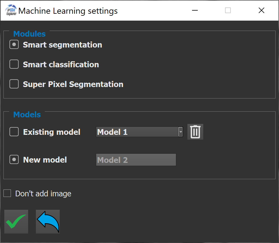
Under the module selection, it is possible to choose between creating or selecting an existing model. The name of the model is editable when creating a new model. Also, an existing model can be deleted by selecting it in the drop-down list and using the trash button.
After using the validate button, the graphical interface of the smart segmentation module shows inside a new window.
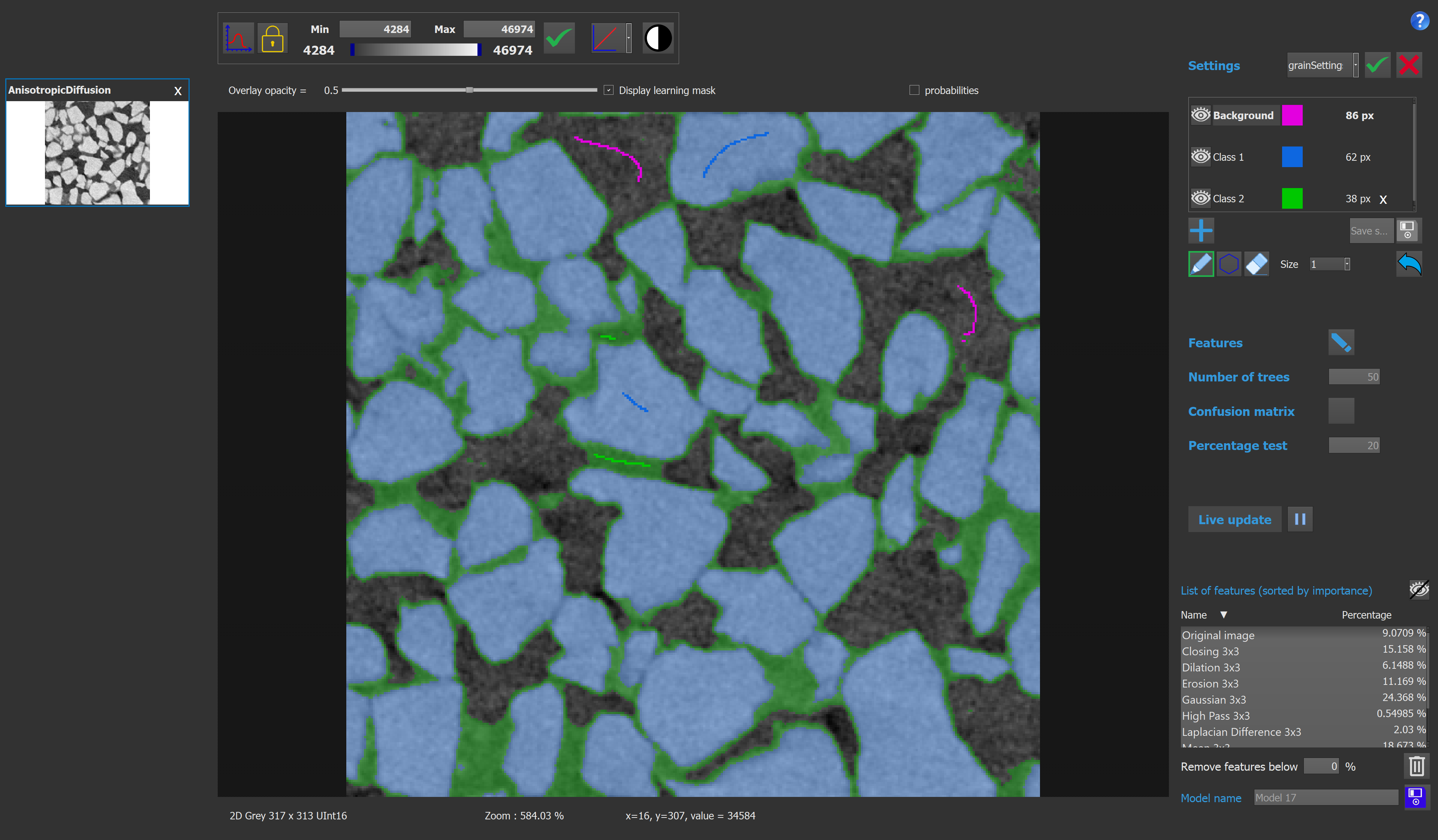
Here is the graphical interface for this module :
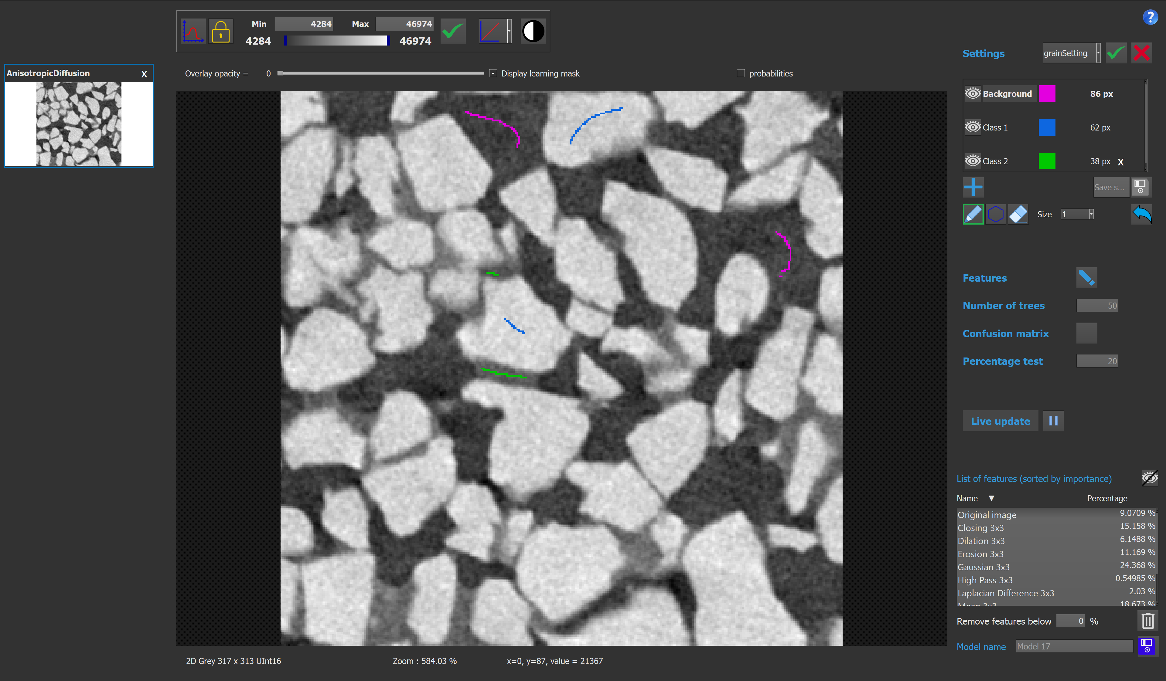
The class selection box contains all the information concerning the classes of the model. The user can add or delete a class, rename it, and also change the color used to visualize a class. If there is only 2 classes on the model, the output image will be binary, otherwise it will be a labeled image. It is possible to change the selected class by clicking on it. Once a class is selected, the user can add pixels to this class by drawing on the image. If the eraser button is activated, drawing on the image will remove pixels from the selected class. The number on the right of each class indicates the number of pixels contained by this class.
The polygon tool can also be used to add pixels to a class. Clicking on the image will add new points to the polygon, while double clicking will close and fill the polygon.
It is possible to delete all the drawings by right clicking on the image thumbnail on the left and selecting "clear draw" in the context menu.
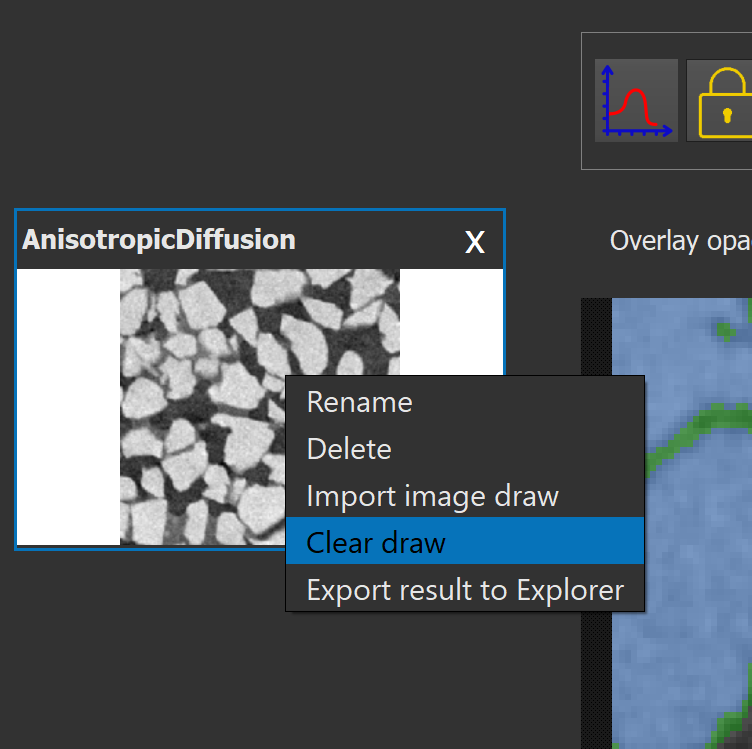
The same menu can be used to export results into the main viewer of Explorer by clicking "Export result to Explorer". Exporting results when working on a 3D image will only export the current plane into Explorer's viewer. Drawings of other models can be imported to the current model by clicking "Import image draw".
Then the user can choose the features for the model. Here each feature corresponds to a process applied on the image. This way we take into account the pixel neighborhood, and only not the value of the pixel.
Here we have the widget used to define the features :
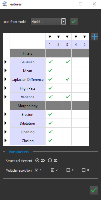
It is possible to load the features settings from an existing model, and apply it to the current model.
On the left column of the table, we have the names of the functions used to compute the features. On the top row, we have the half size of the kernels used in those functions.

Clicking on an arrow will select, or unselect, an entire row or column.
The choice "2D" or "3D" is meaningful only when working with 3D images. In this case, selecting "2D" will apply a 2D kernel plane by plane, and "3D" will apply a 3D kernel on the image.
Each value of multiple resolution will divide the size of the image (by 2, 4 or 8), then apply the feature computation, then go back to the original image size.
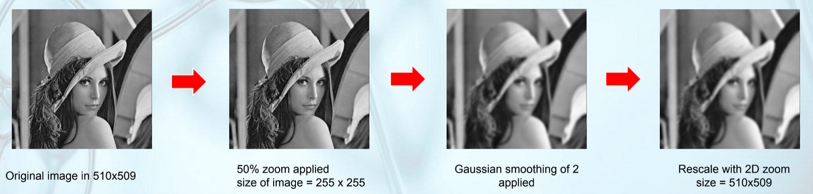
The aim of this process is to take into account a distant neighborhood, without using very large kernel, to avoid a long computation time. For example, applying a Gaussian 3x3 process, with a multiple resolution of 4, will give similar result than directly applying a Gaussian 12x12. But the process will be much faster.
The list of features box shows all the features used in the model. By clicking on a feature, the user can visualize the image corresponding to a feature.
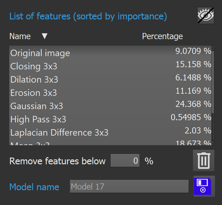
The list can be sorted by names, or by percentages, by clicking on the corresponding column. To stop displaying a feature, the user can click on the eye button.
Once the model is computed, each features will have an associated percentage, which shows how much a feature impacts the model. The functionality "Remove features below %" allows the user to remove the meaningless features. To do so, the user chooses a threshold in percentage, and click on the trash button. The features selection widget will be updated automatically.

A Confusion Matrix [2] is a table used in machine learning and statistics to evaluate the performance of a classification model. It compares predicted values (model outputs) with actual values (ground truth) in a grid format, typically 2x2 for binary classification or larger for multi-class problems.
The actual values are the pixels drawn by the user, while the predicted values are the values predicted by the algorithm on the percentage of pixels used for the test. The pixels used for the test represents a certain percentage given by the user (20% by default).
Each categories of values, between the predicted values and actual values, can be either positive or negative, which results in 4 different outcomes.
The different errors categories includes :
The confusion matrix appears like this inside Explorer :
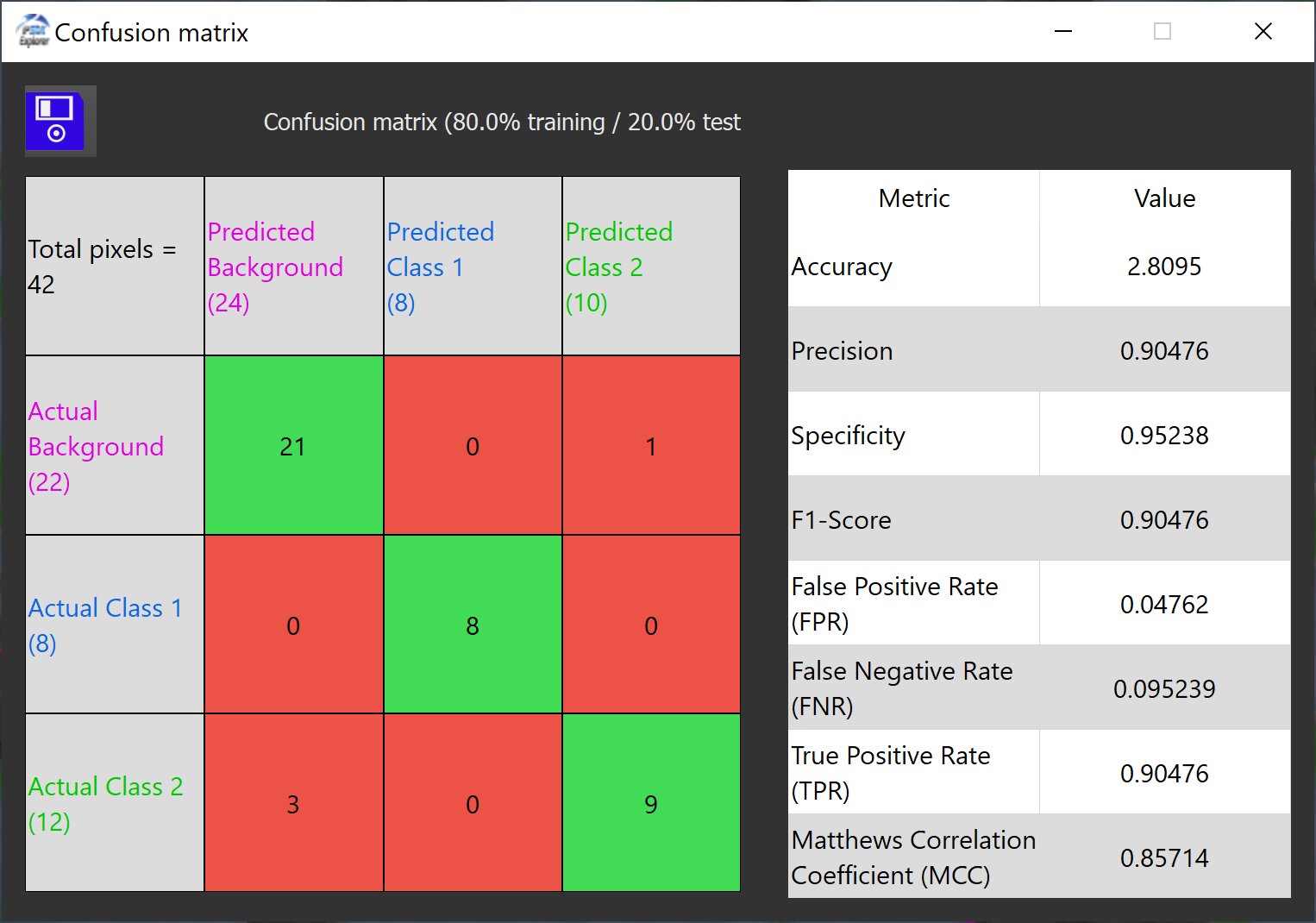
The matrix appears on the left side of the window, while the metrics computed for this matrix shows on the right.
Each metrics gives informations on the classification accuracy of the model. There is 8 different metrics computed.
The accuracy [3] metric measures the overall correctness of the model by calculating the proportion of correctly predicted samples (both true positives and true negatives) out of all samples.
It is defined by the formula :
![\[ \text{Accuracy} = \frac{\text{TP} + \text{TN}}{\text{TP} + \text{TN} + \text{FP} + \text{FN}} \]](IPSDKCore_form_36.png)
The precision [4] metric, also known as Positive Predictive Value, indicates the proportion of true positive predictions out of all positive predictions made by the model. It reflects how precise the model is in identifying positive cases.
It is defined by the formula :
![\[ \text{Precision} = \frac{\text{TP}}{\text{TP} + \text{FP}} \]](IPSDKCore_form_37.png)
The specificity [5] metric, also known as True Negative Rate, measures the ability of the model to correctly identify negative cases out of all actual negative cases. It complements the sensitivity metric (TPR).
It is defined by the formula :
![\[ \text{Specificity} = \frac{\text{TN}}{\text{TN} + \text{FP}} \]](IPSDKCore_form_38.png)
The True Positive Rate (TPR) [5] metric, also known as Sensitivity/Recall, measures the proportion of actual positive cases correctly classified as positive by the model.
It is defined by the formula :
![\[ \text{TPR} = \frac{\text{TP}}{\text{TP} + \text{FN}} \]](IPSDKCore_form_39.png)
The F1-Score [6] metric combines precision and recall (TPR) into a single metric that balances the two. This metric is useful when the data is imbalanced.
It is defined by the formula :
![\[ \text{F1-Score} = 2 \cdot \frac{\text{Precision} \cdot \text{TPR}}{\text{Precision} + \text{TPR}} \]](IPSDKCore_form_40.png)
The False Positive Rate (FPR) [7] metric represents the proportion of actual negative cases incorrectly classified as positive.
It is defined by the formula :
![\[ \text{FPR} = \frac{\text{FP}}{\text{FP} + \text{TN}} \]](IPSDKCore_form_41.png)
The False Negative Rate (FNR) [8] metric represents the proportion of actual positive cases incorrectly classified as negative.
It is defined by the formula :
![\[ \text{FNR} = \frac{\text{FN}}{\text{FN} + \text{TP}} \]](IPSDKCore_form_42.png)
The Matthews Correlation Coefficient (MCC) [9] metric provides a balanced measure that takes into account all values in the confusion matrix (TP, TN, FP, FN). This metric is useful for imbalanced datasets.
It is defined by the formula :
![\[ \text{MCC} = \frac{\text{TP} \cdot \text{TN} - \text{FP} \cdot \text{FN}} {\sqrt{(\text{TP} + \text{FP})(\text{TP} + \text{FN})(\text{TN} + \text{FP})(\text{TN} + \text{FN})}} \]](IPSDKCore_form_43.png)
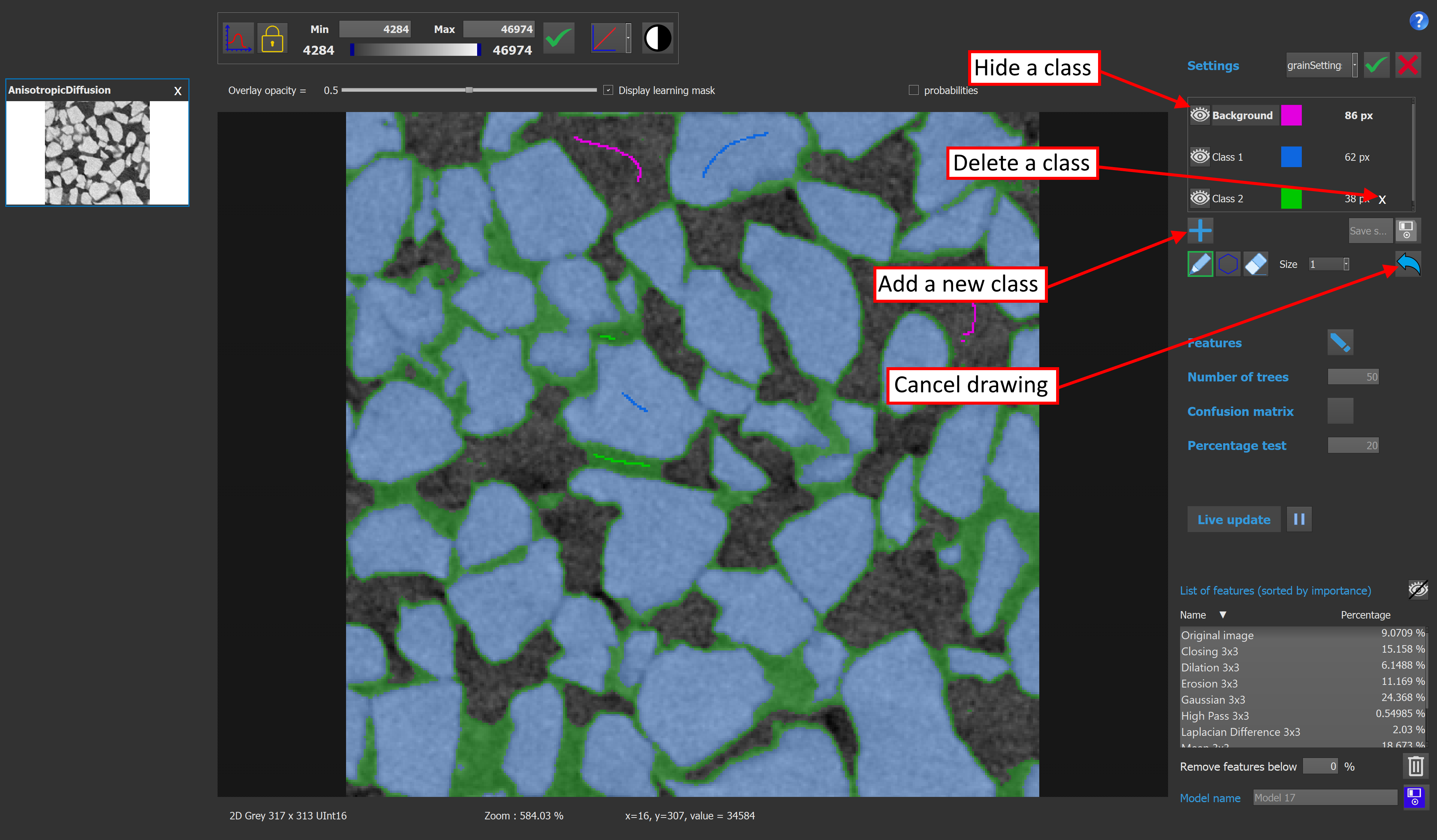
A probability map can be displayed with different luts inside the viewer by clicking the "probabilities" checkbox on the top right corner of the viewer.
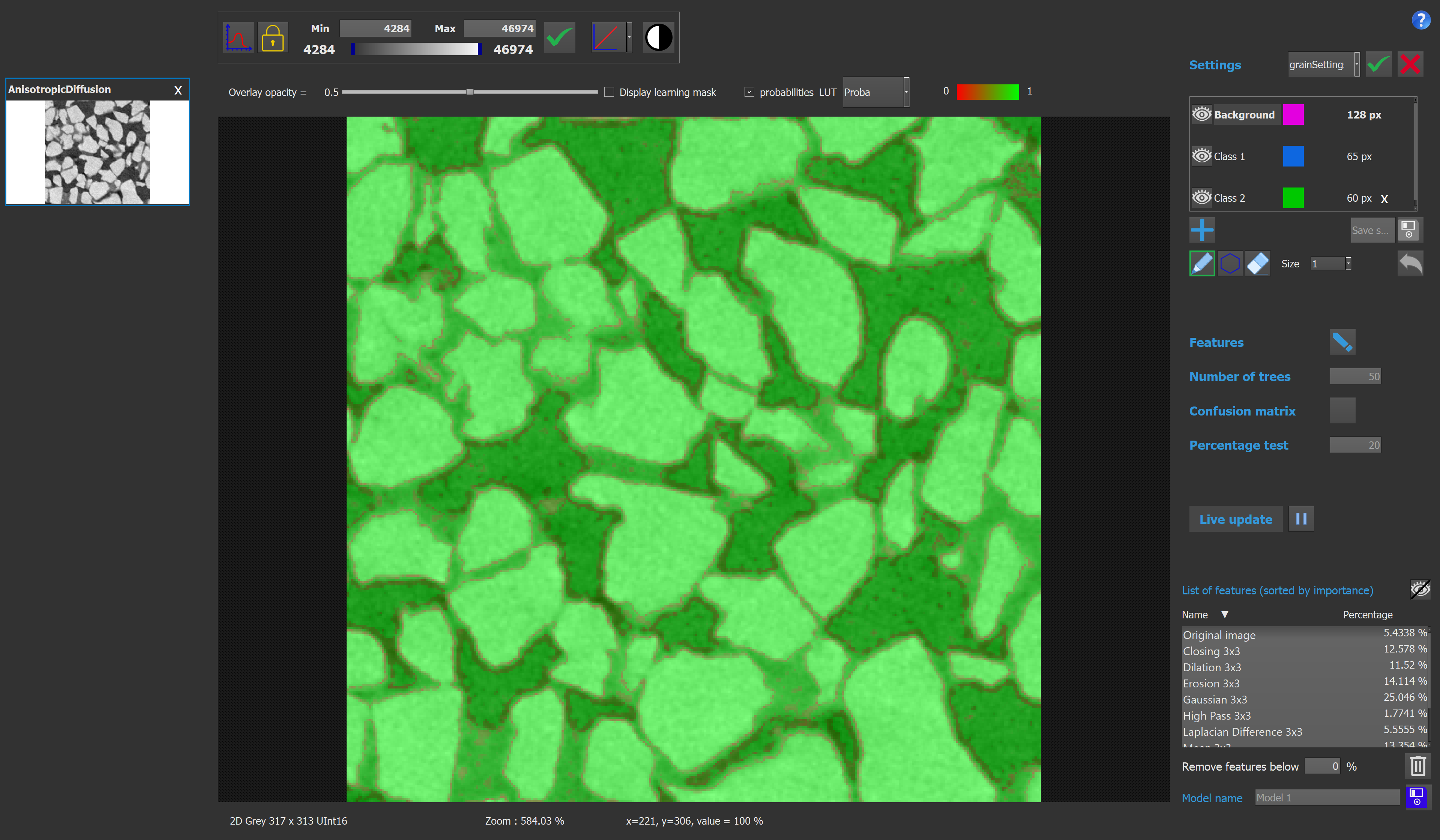
The probability map provides additional information by indicating the reliability with which a pixel has been classified. It is calculated as the ratio of the number of trees that "voted" for the selected class of the pixel to the total number of trees. The higher the value, the more likely it is that the pixel has been correctly classified.
On the main window, the user can also change the number of trees used in the random forest model. With more trees, the model will be more precise, but the computation time will be longer.
It is also possible to activate or deactivate the 'live update' mode. If this mode is activated, the model will be actualized every time a pixel is added to a class, or removed from a class. If this mode is deactivated, the user can actualize the model manually.

Here we have an example of a model with 3 classes. The features setting used to compute this model is the one presented on the previous image.
Once the user is satisfied with the model, it can be saved and used inside Explorer by running the smart segmentation function.
[1] https://en.wikipedia.org/wiki/Random_forest
[2] https://en.wikipedia.org/wiki/Confusion_matrix
[3] https://en.wikipedia.org/wiki/Accuracy_and_precision#In_classification
[4] https://en.wikipedia.org/wiki/Positive_and_negative_predictive_values
[5] https://en.wikipedia.org/wiki/Sensitivity_and_specificity
[6] https://en.wikipedia.org/wiki/F-score
[7] https://en.wikipedia.org/wiki/False_positive_rate
[8] https://en.wikipedia.org/wiki/False_positives_and_false_negatives#false_negative_rate
