Introduction
The geometry characterizes the image properties, carrying :
- the image buffer type,
- the image dimensions.
The available buffer types are :
- UInt8 / Binary / Label8,
- Int8,
- UInt16 / Label16,
- Int16,
- UInt32 / Label32,
- Real32.
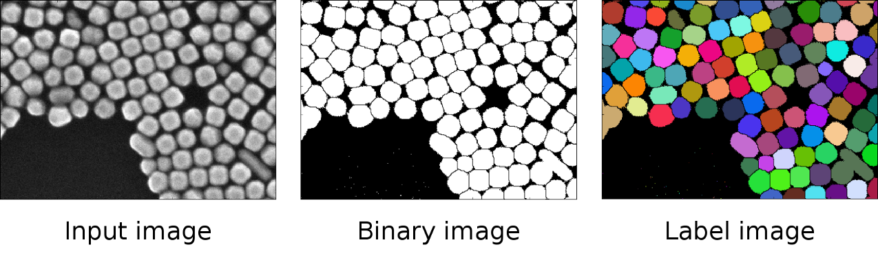
Binary images are unsigned 8-bits data used as logical mask images and its possible values are 0 or 1. As for Label8, Label16 and Label32 images, they have unsigned 8, 16 or 32-bits data type and are used to identify objects in the image by an integer value.
The figure below shows an input image (left), its thresholded and segmented binary version (middle) and the labelled image assigning a label (represented by a color in the image) to the pixels of a blob.
See ipsdk::image::eImageBufferType for more details.
Geometry creation
Functions to create a geommetry
Several functions allow to create a geometry, specifying the required information. Here is the list of these functions :
- ipsdk::image::geometry2d defines the geometry of 2d grey level images,
- ipsdk::image::geometry3d defines the geometry of 3d grey level images,
- ipsdk::image::geometryRgb2d defines the geometry of 2d RGB images,
- ipsdk::image::geometryRgb3d defines the geometry of 3d RGB images,
- ipsdk::image::geometrySeq2d defines the geometry of 2d grey level image sequences,
- ipsdk::image::geometrySeq3d defines the geometry of 3d grey level image sequences.
Functions to reinterpret a geommetry
It is possible to reinterpret an image geometry without creating a new image. For instance, a 3D image can instantly become a multi-channel or a sequence image. The conversion are availeble through the following functions:
- ipsdk::image::reinterpretVolumeToSequence to interpret a volume as a sequence image,
- ipsdk::image::reinterpretSequenceToVolume to interpret a sequence image as a volume,
- ipsdk::image::reinterpretVolumeToMultiChannel to interpret a volume as a multi-channel image,
- ipsdk::image::reinterpretMultiChannelToVolume to interpret a multi-channel image as a volume,
- ipsdk::image::reinterpretSequenceToMultiChannel to interpret a sequence as a multi-channel image,
- ipsdk::image::reinterpretMultiChannelToSequence to interpret a multi-channel image as a sequence.
Please, note that the input image must have 3 dimensions. This means that:
- if the image is 3D, it can't contain several color channels or frames,
- if the image is multi- channel, it can't be a 3D volume or contain several frames,
- if the image is a sequence, it can't be a 3D volume or contain several channels.
Geometry components
We can distinguish three kinds of geometry :
- Volume geometry, which determines if the image is 2d or 3d and is described by ipsdk::image::eVolumeGeometryType,
- Color geometry, which informs if the data is a grey level, RGB, or any other supported color space model, and is described by ipsdk::image::eColorGeometryType,
- Temporal geometry, which allows to handle image sequences, and is described by ipsdk::image::eTemporalGeometryType.
Color models
RGB color model
The RGB color model is associated to the three primary colors :
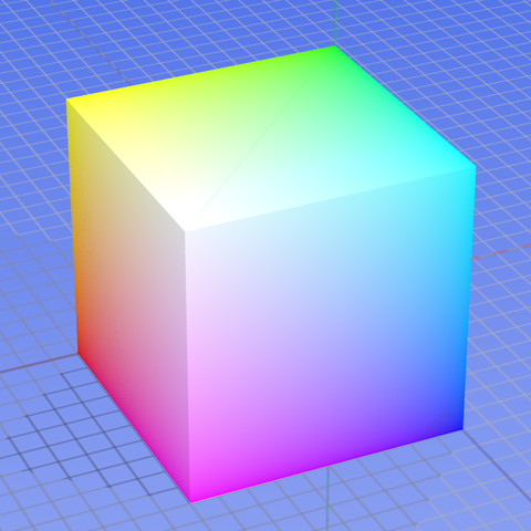
The RGB color model mapped to a cube. The horizontal x-axis as red values increasing to the left, y-axis as blue increasing to the lower right and the vertical z-axis as green increasing towards the top. The origin, black, is the vertex hidden from view.
- See also
- http://en.wikipedia.org/wiki/RGB_color_model
RGBA color model
The RGB color model is associated to the three primary colors :
with an additional Alpha channel which can be used for example to handle transparency.
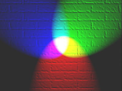
A representation of additive color mixing. Projection of primary color lights on a white screen shows secondary colors where two overlap; the combination of all three of red, green, and blue in equal intensities makes white.
- See also
- https://en.wikipedia.org/wiki/RGBA_color_space
-
http://en.wikipedia.org/wiki/RGB_color_model
XYZ Rec 709 color models
The CIE system is based on the description of color as a luminance component Y, as described above, and two additional components X and Z.
It is defined such that all visible colours (physiologically perceived colors in human color vision) can be defined using only positive values, and, the Y value is luminance. We use the CIE XYZ color space as defined by ITU-R BT.709-6 Recommendation with D65 white point.
The standardized transformation settled upon by the CIE special commission was as follows:
![\[ \begin{bmatrix} X \\ Y \\ Z \end{bmatrix} = \begin{bmatrix} 3.24045 & -1.53714 & -0.49853 \\ -0.96927 & 1.87601 & 0.041567 \\ 0.055643 & -0.20403 & 1.05723 \end{bmatrix} \begin{bmatrix} R \\ G \\ B \end{bmatrix} \]](IPSDKCore_form_254.png)
The inverse matrix is then given by :
![\[ \begin{bmatrix} R \\ G \\ B \end{bmatrix} = \begin{bmatrix} 0.41246 & 0.35758 & 0.18044 \\ 0.21267 & 0.71515 & 0.07218 \\ 0.01933 & 0.11919 & 0.95030 \end{bmatrix} \begin{bmatrix} X \\ Y \\ Z \end{bmatrix} \]](IPSDKCore_form_255.png)
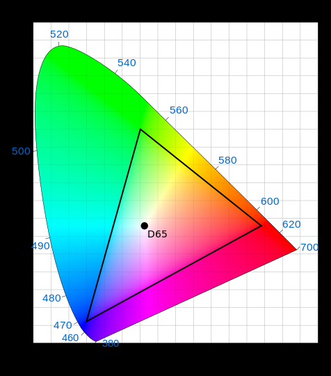
BT.709 primaries shown on the CIE 1931 x, y chromaticity diagram. Colors within the BT.709 color gamut will fall within the triangle that connects the primaries. Also shown is BT.709's white point, Illuminant D65.
- See also
- Digital Video and HD, Algorithms and Interfaces (2nd ed.), Poynton, 2012-02-07.
-
https://fr.wikipedia.org/wiki/SRGB
YCbCr and YPbPr color models
The YCbCr color model defines a color space where :
- Y stands for the luma component (the brightness)
- Cb and Cr are the chrominance (color) components.
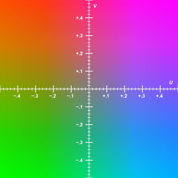
Example of Cb-Cr color plane
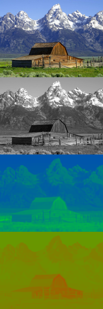
A RGB image along with its Y, Cb, and Cr components respectively.
YCbCr is sometimes abbreviated to YCC and is used in case of digital signal. YPbPr, sometimes called Yuv, is used in case of analog signal.
YCbCr and YPbPr are then closely related since color spaces are linked by following equations :
![\[ \begin{bmatrix} Y \\ C_b \\ C_r \end{bmatrix} = \begin{bmatrix} Y \\ \frac{224}{219} P_b + 2^{n-1} \\ \frac{224}{219} P_r + 2^{n-1} \end{bmatrix} \]](IPSDKCore_form_256.png)
where  stands for the number of the bit length of the quantized signal. Note that
  normalization term is only added in case of unsigned int data type.
The standardized transformation settled upon by the CIE special commission, as defined by ITU-R BT.709-6 Recommendation with D65 white point, is given by :
![\[ \begin{bmatrix} Y \\ P_b \\ P_r \end{bmatrix}_{709} = \begin{bmatrix} 0.2126 & 0.7152 & 0.0722 \\ -0.11457 & -0.38543 & 0.5 \\ 0.5 & -0.45415 & -0.04585 \end{bmatrix} \begin{bmatrix} R \\ G \\ B \end{bmatrix} \]](IPSDKCore_form_258.png)
The inverse matrix is then given by :
![\[ \begin{bmatrix} R \\ G \\ B \end{bmatrix} = \begin{bmatrix} 1.0 & 0 & 1.5748 \\ 1.0 & -0.18732 & -0.46812 \\ 1.0 & 1.8556 & 0 \end{bmatrix} \begin{bmatrix} Y \\ P_b \\ P_r \end{bmatrix}_{709} \]](IPSDKCore_form_259.png)
- See also
- https://en.wikipedia.org/wiki/YCbCr
-
Digital Video and HD, Algorithms and Interfaces (2nd ed.), Poynton, 2012-02-07.
L*a*b color model
This color space were defined by the International Commission on Illumination (CIE) in 1976.
Its three components stand for :
- L* : lightness
- a* : green-red component
- b* : blue-yellow component
These values can be obtained from XYZ Rec 709 color models as follow :
![\[ \begin{cases} L^*=116 f \left( \frac{Y}{Y_n} \right ) - 16 \\ a^*=500 \left( f \left( \frac{X}{X_n} \right ) - f \left( \frac{Y}{Y_n} \right ) \right ) \\ b^*=200 \left( f \left( \frac{Y}{Y_n} \right ) - f \left( \frac{Z}{Z_n} \right ) \right ) \end{cases} \]](IPSDKCore_form_260.png)
where :
![\[ f(t)=\begin{cases} \sqrt[3]{t} & \text{if}\ t>\delta^3 \\ \frac{t}{3\delta^2}+\frac{4}{29} & \text{otherwise} \end{cases}, \delta = \frac{6}{29} \]](IPSDKCore_form_261.png)
and :
![\[ \begin{cases} X_n=0.95047 \\ Y_n=1.0 \\ Z_n=1.08883 \end{cases} \]](IPSDKCore_form_262.png)
The reverse transformation is then given by :
![\[ \begin{cases} X=X_nf^{-1}\left(\frac{L^*+16}{116}+\frac{a^*}{500} \right) \\ Y=Y_nf^{-1}\left(\frac{L^*+16}{116} \right) \\ Z=Z_nf^{-1}\left(\frac{L^*+16}{116}-\frac{b^*}{200} \right) \end{cases} \]](IPSDKCore_form_263.png)
where :
![\[ f^{-1}(t)=\begin{cases} t^3 & \text{if}\ t>\delta \\ 3\delta^2\left(t-\frac{4}{29}\right) & \text{otherwise} \end{cases} \]](IPSDKCore_form_264.png)
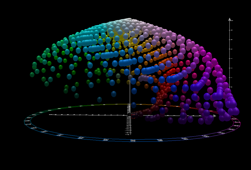
CIELAB color space front view
- See also
- https://en.wikipedia.org/wiki/CIELAB_color_space
-
https://en.wikipedia.org/wiki/Standard_illuminant
-
Digital Video and HD, Algorithms and Interfaces (2nd ed.), Poynton, 2012-02-07.
L*u*v* color model
This color space were adopted by the International Commission on Illumination (CIE) in 1976
Its three components stand for :
- L* : lightness
- u* : first chroma component
- v* : second chroma component
These values can be obtained from XYZ Rec 709 color models as follow :
![\[ \begin{cases} L^*=\begin{cases} \left(\frac{29}{3}\right)^3\frac{Y}{Y_n}, & \text{if}\ \frac{Y}{Y_n}<=\left(\frac{6}{29}\right)^3 \\ 116\left(\frac{Y}{Y_n}\right)^{\frac{1}{3}}-16, & \text{otherwise} \end{cases} \\ u^*=13L^*({u}'-{u_n}') \\ v^*=13L^*({v}'-{v_n}') \end{cases} \]](IPSDKCore_form_265.png)
where :
![\[ \begin{cases} {u}'=\frac{4X}{X+15Y+3Z} \\ {v}'=\frac{9Y}{X+15Y+3Z} \end{cases} \]](IPSDKCore_form_266.png)
and :
![\[ \begin{cases} Y_n=0.329024 \\ {u_n}'=0.1978 \\ {v_n}'=0.4683 \end{cases} \]](IPSDKCore_form_267.png)
The reverse transformation is then given by :
![\[ \begin{cases} {u}'=\frac{u^*}{13L^*}+{u_n}' \\ {v}'=\frac{v^*}{13L^*}+{v_n}' \end{cases} \]](IPSDKCore_form_268.png)
and then :
![\[ \begin{cases} Y=\begin{cases} Y_n L^* \left(\frac{3}{29}\right)^3, & \text{if}\ L^*<=8 \\ Y_n \left(\frac{L^*+16}{116}\right)^3, & \text{otherwise} \\ \end{cases} \\ X=Y\frac{9{u}'}{4{v}'} \\ Z=Y\frac{12-3{u}'-20{v}'}{4{v}'} \end{cases} \]](IPSDKCore_form_269.png)
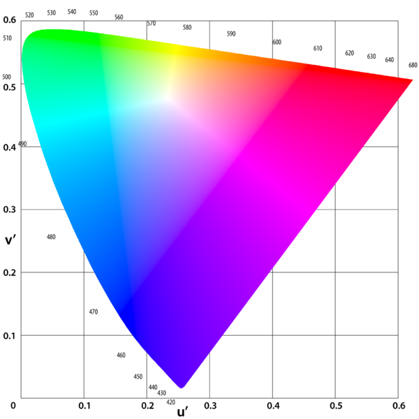
(u', v') chromaticity diagram, also known as the CIE 1976 UCS (uniform chromaticity scale) diagram.
- See also
- https://en.wikipedia.org/wiki/CIELUV
-
https://en.wikipedia.org/wiki/Standard_illuminant
-
Digital Video and HD, Algorithms and Interfaces (2nd ed.), Poynton, 2012-02-07.
HLS color model
HLS color space stands for Hue, Lightness and Saturation color space where :
- Hue is defined technically as "the degree to which a stimulus can be described as similar to or different from stimuli that are described as red, green, blue, and yellow"
- Lightness is the "brightness relative to the brightness of a similarly illuminated white"
- Saturation is the "colorfulness of a stimulus relative to its own brightness"
Transformation from a RGB color model is given by :
![\[ \begin{cases} M=max(R, G, B) \\ m=min(R, G, B) \\ C = M-m \\ {H}' = \begin{cases} 0 & \text{if}\ C=0 \\ \frac{G-B}{C} & \text{if}\ M=R \\ \frac{B-R}{C}+2 & \text{if}\ M=G \\ \frac{R-G}{C}+4 & \text{if}\ M=B \end{cases} \\ H = modulo(60{H}', 360) \\ L=\frac{M+m}{2} \\ S=\begin{cases} 0 & \text{if}\ L=1 \\ \frac{C}{1-\left | 2L-1 \right |} & otherwise \end{cases} \end{cases} \]](IPSDKCore_form_270.png)
On output these components take value in :
![$[0, 1]$](IPSDKCore_form_271.png) for saturation and lightness
for saturation and lightness![$[0, 360]$](IPSDKCore_form_272.png) for hue
for hue
Reverse transformation is then given by :
![\[ \begin{cases} C=(1-\left | 2L-1 \right |) \times S \\ {H}'=\frac{H}{60} \\ X=C \times (1-\left | {H}' \mod 2 - 1 \right |) \\ (R, G, B) = (L-\frac{C}{2}) + \begin{cases} (C, X, 0) & \text{if}\ 0 <= {H}' <= 1 \\ (X, C, 0) & \text{if}\ 1 <= {H}' <= 2 \\ (0, C, X) & \text{if}\ 2 <= {H}' <= 3 \\ (0, X, C) & \text{if}\ 3 <= {H}' <= 4 \\ (X, 0, C) & \text{if}\ 4 <= {H}' <= 5 \\ (C, 0, X) & \text{if}\ 5 <= {H}' <= 6 \\ \end{cases} \end{cases} \]](IPSDKCore_form_273.png)
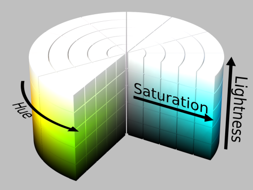
HLS cylinder.
- See also
- https://en.wikipedia.org/wiki/HSL_and_HSV
HSV color model
HSV color space stands for Hue, Saturation and Value color space where :
- Hue is defined technically as "the degree to which a stimulus can be described as similar to or different from stimuli that are described as red, green, blue, and yellow"
- Saturation is the "colorfulness of a stimulus relative to its own brightness"
- Value is the "attribute of a visual sensation according to which an area appears to emit more or less light"
Transformation from a RGB color model is given by :
![\[ \begin{cases} M=max(R, G, B) \\ m=min(R, G, B) \\ C = M-m \\ {H}' = \begin{cases} 0 & \text{if}\ C=0 \\ \frac{G-B}{C} & \text{if}\ M=R \\ \frac{B-R}{C}+2 & \text{if}\ M=G \\ \frac{R-G}{C}+4 & \text{if}\ M=B \end{cases} \\ H = modulo(60{H}', 360) \\ V=M \\ S=\begin{cases} 0 & \text{if}\ V=0 \\ \frac{C}{V} & otherwise \end{cases} \end{cases} \]](IPSDKCore_form_274.png)
On output these components take value in :
- for saturation and value
- for hue
Reverse transformation is then given by :
![\[ \begin{cases} C=V \times S \\ {H}'=\frac{H}{60} \\ X=C \times (1-\left | {H}' \mod 2 - 1 \right |) \\ (R, G, B) = (V-C) + \begin{cases} (C, X, 0) & \text{if}\ 0 <= {H}' <= 1 \\ (X, C, 0) & \text{if}\ 1 <= {H}' <= 2 \\ (0, C, X) & \text{if}\ 2 <= {H}' <= 3 \\ (0, X, C) & \text{if}\ 3 <= {H}' <= 4 \\ (X, 0, C) & \text{if}\ 4 <= {H}' <= 5 \\ (C, 0, X) & \text{if}\ 5 <= {H}' <= 6 \\ \end{cases} \end{cases} \]](IPSDKCore_form_275.png)
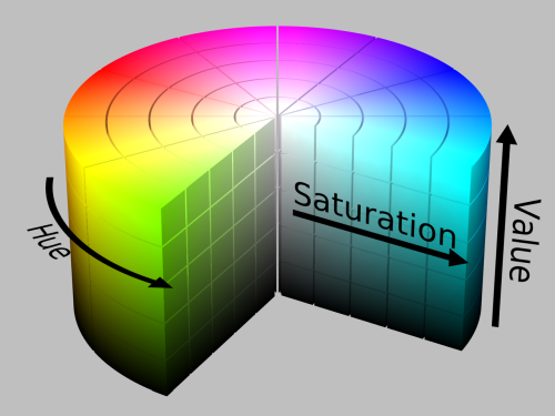
HSV cylinder.
- See also
- https://en.wikipedia.org/wiki/HSL_and_HSV