Image color mapping 2d

image =	colorMapping2dImg (inImg,colorMap)
image =	colorMapping2dImg (inImg,colorMap)
image =	colorMapping2dImg (inImg,pIColorMap)
image =	colorMapping2dImg (inImg,pIColorMap)

Detailed Description

application of a color map on each 2D plan of an input grey-levels image

This algorithm applies a given color map to each 2D plan of an input grey-levels image with voxels values encoded with unsigned integers, in order to make the visualization of the input image easier for the user.

There are mainly two types of color maps that can be used by the algorithm: the cyclic color maps and the smooth color maps.

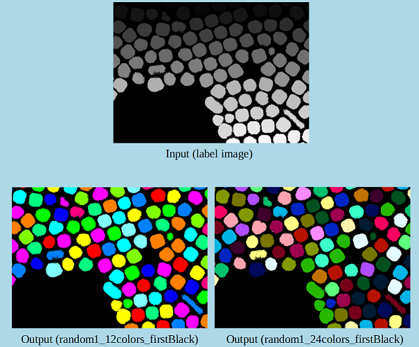
• In cyclic color maps, the table defined in the color map is a collection of Rgb data items, that are triplets of (R, G, B) normalized floating values, between 0 and 1, that define the color to apply. If the number of colors defined in the map is lower than the number of intensities in the input image, the colors to apply to intensities greater than the map size are automatically deduced as the repetition of the table elements. These color maps are typically used to visualize label images, for instance. Depending on the cycle mode chosen by the user, the first color of the map may or may not belong to the cycle. It may be useful in label images where the 0-value is reserved for the background, for instance (in that case, it may be desirable that a specific color may be dedicated for that background).

  To sum it up, given an input image (2D here, for the example) and a specific cyclic color map, values of the color output image will equal to:

  

• In smooth color maps, the table defined in the color map is a collection of AbscissRgb data items. As indicated by its name, this data item is made of an absciss, and a triplet of (R, G, B) normalized floating values, between 0 and 1. First and last colors of the map are respectively applied to min and max, with (min, max) equalling to the minimum and maximum of the input image, or the minimum and maximum of the data type used to encode the values of the pixels of the image, depending on the range mode chosen by the user. Colors to apply to other intensities of the input image are computed by linear interpolation between the color of table that has the closest absciss, that is lower than current intensity, and the element of table that has the closest absciss, that is greater than current intensity. Smooth color maps are typically used to enhance contrast of the image displayed to the user, or to use a code of color that is interpreted more easily by the user.

The user can specify its own customized color map, but IPSDK also provides some predefined color maps, for both types of maps:

• For cyclic maps:
  • Random1_12Colors, cyclic random color map made of 12 different colors
    
  • Random1_12Colors_FirstBlack, cyclic random color map made of 12 different colors; all colors are automatically repeated, except the first one( black)
    
  • Random2_12Colors, cyclic random color map made of 12 different colors
    
  • Random2_12Colors_FirstBlack, cyclic random color map made of 12 different colors; all colors are automatically repeated, except the first one( black)
    
  • Random1_24Colors, cyclic random color map made of 24 different colors
    
  • Random1_24Colors_FirstBlack, cyclic random color map made of 24 different colors; all colors are automatically repeated, except the first one( black)
    
• As for predefined smooth color maps, they are well known by matplotlib users:
  • Jet
    
  • InvJet
    
  • Viridis
    
  • Magma
    
  • Inferno
    
  • Plasma
    

Here are different examples of predefined cyclic color maps applied to a label image:

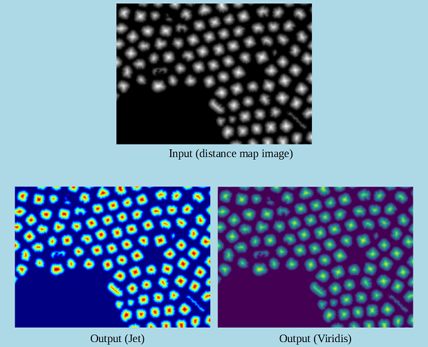
And here are different examples of predefined smooth color maps applied to Lena grey levels image:

Example of Python code :

Example imports

import PyIPSDK
import PyIPSDK.IPSDKIPLIntensityTransform as itrans

Code Example

    # opening of input images
    inImg = PyIPSDK.loadTiffImageFile(inImgPath)
    
    # application of color map on input image (1st signature test)
    outImg = itrans.colorMapping2dImg(inImg, colorMap)

Example of C++ code :

Example informations

Header file

#include <IPSDKIPL/IPSDKIPLIntensityTransform/Processor/ColorMapping2dImg/ColorMapping2dImg.h>

Code Example

    ImagePtr pInImg = loadTiffImageFile(inImgFilePath, eTiffDirectoryMode::eTDM_Volume);
    const CyclicRgbColorMapPtr pColorMap =
        createCyclicRgbColorMap(ePredefinedCyclicRgbColorMapId::ePCRCMI_Random1_12Colors);
    ImagePtr pOutImg = colorMapping2dImg(pInImg, pColorMap);